Carbon model details
This article provides detailed information about the carbon model. As with the nutrient models, the aim of this model is to strip away much of the complexity of the real ocean and its component ecosystems in order to focus on the key processes that influence the carbon cycle in the ocean.
Overview
The model is physically simple but biogeochemically more advanced than the nutrient models. This model is again intended to be a "minimum complexity" model; it is stripped down to the simplest physical structure that can still give a reasonable representation of the most important aspects of how the ocean’s carbon cycle works. The model is a box model and includes the fluxes of both organic carbon and also calcium carbonate (CaCO3). Dissolved inorganic carbon (split into its two main isotopes) and alkalinity are transported around the model, and carbon is dynamically exchanged with CO2 in the atmosphere.
Aims of this model include:
To understand how the carbonate compensation process works in regulating carbon and climate
To understand how the ocean’s carbon cycle is responding to global change
Carbon cycle
The ocean carbon cycle is considerably more complicated than the cycles of phosphorus, nitrogen and silicon, and this carbon model is therefore inevitably more complex, despite trying to keep things simple.
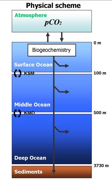
This model is, like the nutrient models, a box model, and like these it does not represent horizontal space at all. It consists of three vertically-stacked boxes, one more than in the ocean nutrient models (see figure to right). The surface box (0-100m) represents the strongly-stirred surface mixed layer which also receives enough sunlight to support growth of phytoplankton. A middle box (100-500m) represents the rest of the annually mixed layer, and a deep box (500-3730m) represents the rest of the deep ocean below the depth of influence of even the strongest waves in winter. Also similarly to the nutrient models, the carbon model has open boundaries that material can cross: it is what is known as an open-system rather than a closed-system model.
The addition of a third box allows both air-sea gas exchange and also mixing with the deep box to be modelled more accurately. Differences between the depth profiles of CaCO3 dissolution and of organic matter remineralisation are also easier to represent (albeit still in a rudimentary way) with three boxes.
The carbonate system
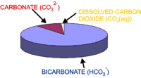
The relative partitioning of DIC into HCO3- ions, CO32- ions and dissolved gas (CO2(aq)) under standard conditions. Most DIC (about 90%) is occurs as HCO3- ions, with only a small fraction (about 1%) as CO2 that can exchange with the atmosphere.
The carbonate system in seawater is the name given to the system of different forms of dissolved inorganic carbon (DIC) in seawater, together with associated variables.
DIC is made up of three different chemical species: dissolved CO2 gas (CO2(aq), the only form able to exchange across the sea-surface), bicarbonate ions (HCO3-) and carbonate ions (CO32-). This system as a whole has two degrees of freedom, and so concentrations of all three species can be calculated from knowledge of any two variables of the carbonate system. The model therefore needs to simulate only two variables. In common with other models, the two that are chosen are DIC and alkalinity (≈ [HCO3-] + 2*[CO32-]).
The distribution of DIC between its three forms, the seawater pH, and the partial pressure of CO2 (pCO2) as well as its concentration ([CO2(aq)]), are all calculated from DIC and alkalinity using routines written by Richard Zeebe and Wolf-Gladrow.
Air-sea gas exchange
The flux of CO2 into and out of the ocean occurs by diffusion across the air-sea interface. This process is modelled using a simple formulation similar to that used in other models. The rate of diffusion is calculated from the difference in partial pressures of CO2 between the sea and the air, and a "transfer velocity".
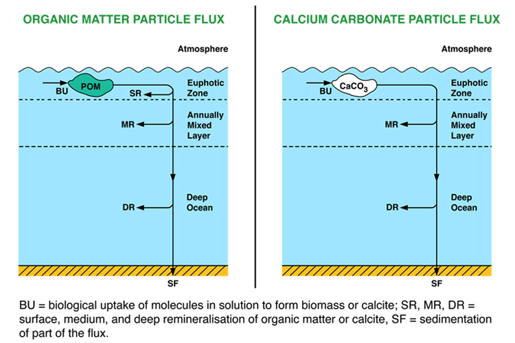
The organic matter pump
Biological uptake of nutrients and CO2 by phytoplankton during photosynthesis and the subsequent remineralisation of sinking detritus throughout the water column creates vertical concentration gradients of DIC and phosphate, with depleted surface waters and enriched deep waters. It is generally accepted that nitrogen and phosphorus are selectively extracted by bacteria from sinking particles compared to carbon and so, therefore, proportionately more carbon gets buried in the sediments compared to the original composition of the sinking particles. Phosphate is taken as the limiting nutrient for primary productivity, in keeping with other similar models. The representation of phytoplankton and its limitation by phosphate is similar to that described in the phosphorus model. The strength of the organic carbon pump in the model is therefore dependent on the supply of new phosphate to the surface box.
Formation of calcium carbonate
Certain species of phytoplankton and zooplankton produce shells made of calcium carbonate, CaCO3, which they precipitate from dissolved calcium and bicarbonate or carbonate ions. Counter-intuitively, the precipitation of CaCO3 increases the concentration of CO2(aq) in seawater:
Ca2+ + 2HCO3- ---> CaCO3 + H2O + CO2
The production of CaCO3 in the surface ocean is linked to the production of organic matter through the ‘rain ratio’ (RR) which is the molar ratio of CaCO3 C export from the surface layer to particulate organic carbon (POC) C export. A significant fraction of CaCO3 formation in reality takes place in coral reef settings in shallow water. This is not treated in any great detail in this model. The focus is on CaCO3 cycling in the open (deep) ocean.
Calcium carbonate cycling
Globally integrated hyspometry.
The model simulates a horizon analogous to ‘snow lines’ on mountains on land, but for CaCO3 deposition in the sea. The colour of marine sediments changes with depth according to the presence/absence of CaCO3. CaCO3 dissolves out of deeper sediments because deeper water is more corrosive for CaCO3. The CaCO3 in seafloor sediments can be of either of two main mineral forms: calcite (usually the most abundant form) or aragonite. The seafloor depth at which calcite CaCO3 disappears from the sediments is known as the carbonate compensation depth (CCD) and the depth at which aragonite starts to disappear as the aragonite compensation depth (ACD). The model simulates only one mineral form of CaCO3; it is all treated as calcite.
The CCD is not fixed but instead is able to vary in response to changing ocean chemistry. For instance, the CCD is set to shallow dramatically as the deep ocean becomes more acidic as fossil fuel CO2 increasingly penetrates to the deep ocean. Because the CaCO3 ‘snow line’ (the CCD) can move up or down in the ocean, the amount of CaCO3 that gets buried depends not only on the intensity of the rain of CaCO3 particles down from the surface layer, but also on the fraction of the seafloor currently allowing accumulation. Or, in other words, it also depends on the fraction of the seafloor that does not dissolve all the CaCO3 that arrives there.
In order to calculate this relationship, ocean hypsometry data is needed. This is the relationship between seafloor depth and fraction of the seafloor situated above that depth (as can be seen in the figure to the right, seafloor is not evenly distributed between different depths). This was obtained from the ETOPO5 dataset of seafloor bathymetry at 5x5 minute resolution across the global ocean. The relative fractions of ocean area at different depths were calculated by summing over the dataset (counting how many points on the global seafloor lie above each depth, and how many below). The critical carbonate ion concentration ([CO32-]c) below which seawater is undersaturated (below which CaCO3 will dissolve) is a function of depth, because increasing seawater pressure makes seawater more corrosive to CaCO3. The model uses the following equation:
to calculate the depth at which ([CO32-]c = [CO32-]). The ocean hypsometry is then used to calculate the fraction of ocean area above or below the CCD, and hence the proportions of the global sinking CaCO3 flux which are buried or dissolved.
Carbon isotopes
Many users will choose to run these models without considering or caring about isotopic ratios, which is perfectly fine. For many purposes there is no need to know about them. However, for the benefit of more advanced users (including palaeoceanographers) the carbon in each reservoir (DIC in each ocean box, and CO2 in the atmosphere) is modelled using two separate variables, one to represent the amount of 12C and one to represent the amount of 13C. So, for instance, 12CO2(aq) and 13CO2(aq) in the surface ocean exchanges with atmospheric reservoirs of 12CO2 and 13CO2. Although the model tracks concentrations of 12C and 13C, results are always presented in terms of concentrations of total carbon (sum of 12C+13C) and d13C values.
When making their CaCO3 shells, foraminifera tend to take up the two isotopes of carbon at more or less the same ratio as they exist in seawater. The ratio is slightly affected however by so-called “vital effects”. Evidence from culture experiments suggests a significant effect of seawater carbonate ion concentration ([CO32-]) on the stable isotope composition of foraminifera. This aspect was also taken into account in our model by using the equation (taken from the scientific literature):
When phytoplankton extract dissolved carbon from seawater during photosynthesis, they discriminate strongly between the two isotopes. Again, however, the degree of discrimination is found to be sensitive to the chemistry of the seawater (as well as other factors). We include the CO2 effect in our model by using the following equation, again taken from the literature:
State variables and equations
Sea surface distribution of DIC. Image by Andy Yool
The following tracers are transported around the model ocean: inorganic phosphate (PO4), phytoplankton (surface box only, expressed separately in units of phosphorus, 12C and 13C), DI12C, DI13C and alkalinity. 12CO2 and 13CO2 are also modelled in the atmosphere, giving rise to a total of 17 state variables. The differential equations are solved using a 4th order Runge-Kutta algorithm. Mass balance checks are carried out to verify that the total numbers of moles of phosphorous, carbon and alkalinity are conserved in the system, after taking into account cumulative inputs (via rivers and fossil fuels) and outputs (via burial) to the system as a whole.
Some brief details of the model equations are given here. Phytoplankton and phosphate are represented in a similar way to the phosphorus model, but expanded here to three boxes. The distribution of CO2(aq) (dissolved inorganic carbon in the form of dissolved CO2 gas, as opposed to bicarbonate or carbonate ions) within the ocean is a function of temperature, salinity, pressure, alkalinity and DIC. The equations used to model alkalinity and DIC are based on the following:
SMS(Alkalinity) = 2* SMS(CaCO3) - SMS(N)
SMS(DIC) = rc/p SMS(P) + SMS(CaCO3)
where SMS is "sources minus sinks" and rc/p is the Redfield ratio of carbon to phosphorus in organic matter. The cycling of nitrate is tied to the cycling of phosphate by Redfield ratios so SMS(N) can be rewritten as rn/p SMS(P). Note that formation of 1 mole of CaCO3 reduces alkalinity by 2 moles but DIC by only 1 mole.
More information about the model construction (before a dynamic CCD was added) is given in a paper looking at how the ocean C sink may change in the future (ref. 1). This model has also been used to explore what will happen to atmospheric CO2 in the long-term after emissions cease (ref. 2). An extended variant of this model has been used to simulate ocean biogeochemical behaviour during the Eocene-Oligocene (ref. 3)).
Fossil-fuel CO2 emissions
Historical (to 2000) and future IPCC SRES CO2 emissions scenarios (to 2100).
The model allows the user to burn coal, oil and gas and add the emitted CO2 to the atmosphere. This can be done either in a simplified way, by adding the CO2 in the form of a sine-wave, or by using historical emissions (generated using records from power stations, cement factories, etc) together with IPCC SRES scenarios. These scenarios represent some possible trajectories of emissions into the future.
Chuck, A. et al. (2005). The oceanic response to carbon emissions over the next century: investigation using three ocean carbon cycle models. Tellus B 57, 70-86.
Tyrrell, T. et al. (2007). The long-term legacy of fossil fuels. Tellus B 59, 664-672.
Merico, A. (2008). Eocene/Oligocene ocean de-acidification linked to Antarctic glaciation by sea level fall. Nature, in press.