Carbon model cons

You wouldn’t use a chain-saw to cut a slice of bread, or a bread-knife to fell a tree. Similarly in modelling, it’s important to choose the most appropriate model for the particular question being addressed. Due to the simplifications made, this model will not be the most appropriate one for some applications. This article describes some of the carbon model cons.
Types of Models
In computer modelling there is a continuum between two caricature classes of models:
- conceptual-type models that aim to simplify a system down to include only its most important elements, in particular those that govern its behaviour
- simulation-type models that are highly detailed and try whenever possible to avoid making assumptions about what is important; instead they try to include as much detail as possible in the expectation that nothing important will be omitted
By simplifying to only the most important fluxes and state variables, this model is very much a conceptual-type model.
Disadvantages
Potential weaknesses of a conceptual approach include the likelihood of omitting something important. Every assumption runs the risk of being incorrect in an important way and thereby divorcing the model results from reality. It only takes one unreasonable assumption or omission, if it relates to a key part of the system, to invalidate the model's results.
Some of the major simplifications and omissions made in the carbon model are as follows:
Lack of spatial resolution: the physical structure of this model consists of three boxes stacked vertically one above the other. It is therefore slightly more complicated than the P, NP and SiP models, which consist of only two boxes. However, there is again no ability to represent any horizontal differences. For this reason this model is inappropriate for looking at regional changes in carbon cycling. The model is suitable only for calculating average global responses.
It also means that this model will not be the best tool for exploring palaeo events during which the ocean circulation underwent significant reorganisation (e.g. a shift in the location of deep-water formation from the high-latitude North Atlantic to the high-latitude North Pacific or the Southern Ocean).
Because of the lack of horizontal resolution this model cannot simulate the solubility pump in the ocean. The solubility pump arises out of the fact that it is cold waters that sink to the ocean depths, and cold waters usually hold more dissolved gases (such as CO2) than do warm waters. This pump a secondary cause of the vertical gradients in carbonate chemistry that are observed in the oceans.
Lack of explicit sediments: some ocean biogeochemical models have a separate part devoted purely to sediments, in which the vertical profiles of sediment material and pore-water chemistry are represented. Processes such as burrowing of worms, decay of organic matter, dissolution of calcium carbonate, etc, are explicitly calculated in each vertical millimetre of sediment. This model does not do that.
This lack prevents modelling of the process of carbonate “burn-down”. If, as is starting to happen at present, deep-water pH falls over time, previously deposited CaCO3 can potentially be dissolved many years after it originally fell to the seafloor, because the overlying waters are becoming increasingly corrosive over time. Because of this lack, our model is likely to respond too slowly at times when the ocean is becoming more acidic. On the other hand, CaCO3 burn-down increases the speed of response to acidification, but does not alter the eventual end-point. The model will converge to the same eventual end-point through the carbonate compensation feedback, but without CaCO3 burn-down will reach it more slowly than it should.
The lack of explicit sediments also prevents the model from representing any decoupling between bottom-water chemistry and sediment pore-water chemistry. This could arise if, for instance, organic matter is being rapidly respired into the sediments, which would make the pore-water more acidic. This omission from the model probably doesn’t introduce any large-magnitude errors.
The model does not represent calcite and aragonite separately. Coccollithophores and foraminifera secrete the calcite polymorph of CaCO3 when building their shells. Pteropods and coral reefs synthesise the aragonite polymorph. The two polymorphs have different solubilities (i.e. different susceptibilities to dissolution). Some organisms also form shells made of high-magnesium calcite, which again has a different solubility from the more usual form. Biological CaCO3 therefore consists of a spectrum of different materials with different dissolution characteristics, but none of this is represented in the model. In the same water-column, for instance, aragonite dissolves much higher up than does calcite (the compensation depths differ).
Related to this last omission, in reality calcite starts to dissolve at the calcite lysocline and then finally disappears altogether from the sediments at the calcite compensation depth. In-between the sediments have intermediate calcite contents. In the model this is all simplified to a sharp transition at one depth. The sediments therefore change from 100% to 0% CaCO3 at the single CCD.
There are uncertainties in the numbers produced by the model due to uncertainties in the carbonate chemistry constants used in the model, although the size of the associated uncertainties is fairly small compared to most other factors.
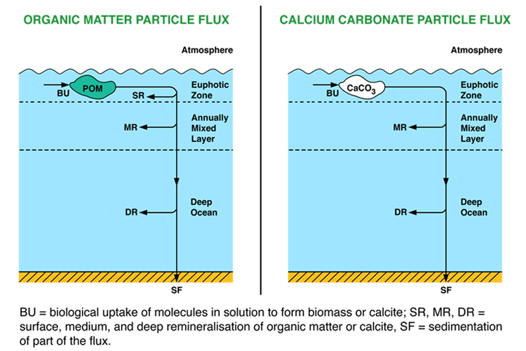
The production of CaCO3 in the surface layer (proportional to POC production) is extremely crude. Populations of coccolithophores, foraminifera, pteropods, etc are not represented as separate variables in the model. In any case we do not understand at all well how their population densities are controlled, and so it is not yet possible to code this accurately into models.
Shallow-water calcification is extremely simplified. Although in reality it accounts for a large fraction of overall CaCO3 burial in the global ocean, in the model it is represented as just one number.
The model includes the delivery of carbon and alkalinity from the land to the oceans, via rivers, but does not include any explicit representation of the weathering processes responsible in part for producing those fluxes. There is no link between climate (atmospheric CO2) and river fluxes.
Only one feedback is included in the model – carbonate compensation. Other potential feedbacks, for instance those associated with silicate or carbonate weathering, are not included.
the terrestrial carbon cycle is not explicitly included as a carbon sink. To date the extra CO2 has been acting as a fertiliser for growth of plants on land, as a result of which extra CO2 has been taken up. The terrestrial biota may, however, according to some predictions, turn into a source of CO2 in the future. Its complete omission will bias atmospheric CO2 projections of the model.
the atmosphere is modelled as a single box; variations with height are not simulated.
the representation of CO2 flux across the sea-surface is done in a simple way that does not included, for instance, the strong dependence on wind-speed. Variations in factors such as windspeed are considered to equal out over the timescales of these model runs.
The model also shares the same simplifications in the representations of biology and phosphate as described for the P-only model.
